Why Flexible Arms Need Stiffness Compensation Calibration
Collaborative robots rely on lightweight, low-stiffness structures to ensure safe human-robot interaction, which makes it difficult to guarantee end-effector accuracy. The body's elastic deformation varies with load and posture, and geometric calibration can only correct fixed parameters such as link lengths and zero positions — it cannot describe this dynamic characteristic. The result is a common phenomenon: the laser tracker fits the model very well, yet the measured end-effector accuracy can hardly reach 3 mm.
The traditional approach — manually teaching points and aligning tip-to-tip — has three inherent shortcomings:
- Geometry only, no deformation: the calibration result is only valid near the sampled points; deformation errors elsewhere in the workspace remain;
- Manual point collection is time-consuming and uneven: uneven distribution of measurement points directly affects calibration quality, and a full calibration typically takes a whole day;
- Calibration is disconnected from operation: third-party calibration equipment and the control system's parameters are not interoperable, so calibration results cannot take effect during operation.
NexAutoCali stiffness compensation calibration replaces this entire workflow: measurement points are generated automatically, the robot runs automatically, and the algorithm identifies parameters automatically. The compensation model is written directly into the iNexBot controller and takes effect in real time with motion control.
Solution Overview
A laser tracker measures the robot's actual end-effector positions under multiple postures and load conditions; the algorithm identifies the stiffness parameters of each joint and arm link and builds a "load → deformation" compensation model; the model is written into the iNexBot controller, which compensates for the deformation of the current posture in real time during motion control.
Compensation Principle
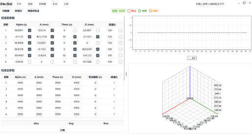
This solution uses a joint-flexibility model: the robot is modeled as rigid links + flexible joints, with the elastic deformation of a joint proportional to the applied torque:
Δx = J(q) · K⁻¹ · (τ_g(q) + τ_load)
where J(q) is the Jacobian matrix, K is the joint stiffness matrix (2 stiffness parameters each for the 6 joints + base, 14 in total; 7-axis models extend to 7 joints + base, 16 in total), τ_g(q) is the gravity torque, and τ_load is the load torque. The algorithm identifies K using weighted least squares, with identification data from measurement points across multiple postures and load conditions to ensure the stiffness parameters are observable.
Two key engineering prerequisites:
- Multi-load excitation: collecting data only under no-load conditions can only identify parameters related to self-weight deformation; stiffness related to user loads cannot be identified. This solution collects data under at least two conditions — no load and rated load (the load model parameters are entered by the user, or obtained by dragging the end-effector during drag teaching and having the system identify the load mass and center of mass);
- Independent validation: a separate validation point set is defined in addition to the identification points, and the report includes the validation results to prevent model overfitting.
The applicable operating condition is quasi-static motion (speed ≤ 500 mm/s). High-speed dynamic deformation, joint backlash, and severe thermal deformation are outside the scope of this compensation model and are handled by the joint-clearance measurement solution and mechanical maintenance procedures respectively. For processes such as polishing where the linear speed may exceed 500 mm/s, we recommend first assessing whether the actual speed falls within the compensation range; anything beyond it should be ensured through mechanical and process means.
Measured Data
Using a flexible arm (rated load 3 kg, speed 500 mm/s) as an example:
| Metric | Before calibration | After calibration |
|---|---|---|
| Position accuracy (AP, 50 measurement points in the workspace, 90th percentile) | 3.0 mm | 0.5 mm |
Error reduced by 83% (accuracy improved 6×). The data is from internal testing under the following conditions: rated load, speed ≤ 500 mm/s, 50 measurement points in the workspace, 90th percentile value.
Technical Specifications
| Item | Specification |
|---|---|
| Measurement equipment | API Radian Plus / Pro / Core laser tracker |
| Tracker accuracy | ±10 µm + 5 µm/m (per the manufacturer's datasheet) |
| Calibration process | Automatic measurement point generation → automatic robot motion → automatic measurement → algorithm identification → parameter writing |
| Calibration duration | 50-point geometric calibration ≤ 5 minutes; full-parameter calibration including stiffness identification 15-30 minutes |
| Full performance verification | 14 metrics per GB/T 12642—2013, approx. 1-2 hours |
| Compensation effect | Compensation calculated within one control cycle, latency < 1 ms |
| Supported models | 7-axis collaborative (CBCBABC), 6-axis collaborative (CBBBAC), etc. |
| Environmental requirements | Ambient temperature 20 ± 2 °C; robot warmed up for 30 minutes before calibration |
| Data confidentiality | Offline mode supported; measurement data never leaves the factory |
Key Advantages
Time: Calibration Reduced from a Full Day to Minutes
- Quick-mount structure: 5 minutes for mechanical connection and software startup (coordinate system alignment and tracker warm-up are additional);
- Measurement points generated automatically and the robot runs automatically — no manual point teaching;
- 50-point geometric calibration ≤ 5 minutes; full-parameter calibration including stiffness identification 15-30 minutes.
Accuracy: Real-Time Compensation at the Control Layer
- Full-parameter calibration covers the main error sources including geometric errors and stiffness deformation;
- Compensation parameters are written directly into the iNexBot controller, and compensation is calculated within one control cycle (latency < 1 ms);
- Measured: position accuracy improved from 3.0 mm to 0.5 mm.
Maintainability: Accuracy Degradation Is Predictable, Maintenance Can Be Scheduled
- Calibration parameters and historical test reports are archived to build an accuracy record for each individual unit;
- Periodic re-testing compared against the historical baseline identifies parameter drift trends and allows maintenance to be scheduled in advance;
- After a controller or mainboard replacement on the same robot, calibration parameters can be restored from backup in minutes; replacing the body (arm links, joints) requires full recalibration.
Applicable Scenarios
| Scenario | Typical process | Expected benefit |
|---|---|---|
| High-precision loading/unloading | CNC loading/unloading, injection molding part extraction | Positioning accuracy stable within 0.5 mm; for changeovers with the same tool and load, the workpiece coordinate system can be established directly on the calibrated TCP, significantly reducing on-site commissioning time |
| Precision assembly | Precision insertion, lamination press-fitting | Force control combined with position accuracy delivers more consistent assembly |
| Polishing | Constant-force polishing, deburring | With trajectory deformation compensation, polishing paths are stable and surfaces consistent (note: applicable to polishing at linear speeds ≤ 500 mm/s; high-speed polishing requires evaluation) |
| Research and education | Robot accuracy experiments, algorithm validation | Provides quantifiable accuracy assessment data and test reports |
Note: the quantitative benefits for assembly and polishing scenarios (e.g., the variation range of insertion force) are currently stated as expectations and will be supplemented with measured data after customer validation.
Why Choose NexAutoCali
- Same-source control and calibration: iNexBot motion control and the calibration algorithm share the same body modeling parameters; calibration results are written directly into the controller and take effect in real time, eliminating parameter compatibility issues;
- A complete measurement-control loop: the solution includes an API high-precision laser tracker, the iNexBot laser measurement system (robot calibration system and robot performance testing system), and the iNexBot control system, with technical support provided uniformly by iNexBot;
- A validation system compliant with national standards: built-in testing of 14 performance metrics per GB/T 12642—2013 "Industrial Robots — Performance Test Methods" (corresponding to ISO 9283:1998); the report can serve as an acceptance basis;
- Continuous model expansion: currently adapted to 7-axis collaborative (CBCBABC) and 6-axis collaborative (CBBBAC) models, with other models under adaptation. Model codes denote the joint configuration by axis sequence (C/B/A correspond to different joint arrangements; e.g., CBCBABC is a 7-axis configuration). See the product brochure for specific load ratings and the adaptation list.
Customer Case
A Collaborative Robot OEM · Assembly Line Application
- Equipment: 6 six-axis collaborative robots for small-part assembly;
- Problem: position accuracy of 2.8 mm after no-load calibration, degrading to 4.5 mm after a load change; changeovers required re-teaching;
- Solution: full-parameter calibration (no-load + rated-load dual conditions), with compensation parameters written into the controller;
- Result: position accuracy reduced to within 0.5 mm; changeovers with the same tool require no re-teaching, and on-site commissioning time was reduced by about 70%;
Implementation Process
- Environment preparation: install the laser tracker and connect the robot; mechanical connection and software startup take about 5 minutes; tracker warm-up and coordinate system alignment are additional (allow ~30 minutes);
- Automatic point generation: the system automatically connects to the robot, reads robot parameters, and automatically plans measurement points (avoiding singularities, limits, and self-collision);
- Automatic measurement: the robot runs automatically through the planned points (no-load + rated-load conditions) while the laser tracker measures actual positions synchronously;
- Stiffness identification: the algorithm identifies geometric parameters and the stiffness compensation model, verified with an independent validation point set;
- Parameter writing: compensation parameters are written into the iNexBot controller and take effect in real time within the control cycle;
- Validation report: performance testing per GB/T 12642—2013, with a before/after calibration comparison report.
Deliverables
- Post-calibration position accuracy test report (before/after comparison, including measurement conditions);
- Stiffness compensation parameter set (written into the controller);
- 14-metric performance test report (Word format);
- Accuracy record (historical reports archived for subsequent re-testing comparison).
FAQ
What is the difference between stiffness compensation calibration and ordinary geometric calibration? Geometric calibration only corrects fixed parameters such as link lengths and zero positions; stiffness compensation additionally identifies deformation characteristics related to load and posture, solving the problem of "accuracy changes when the load or posture changes." For flexible arms, geometric calibration is the foundation, while stiffness compensation is the key to keeping accuracy stable at the 0.5 mm level.
Does recalibration become necessary after changing the fixture or load? Yes. When the load model parameters (mass, center of mass, inertia) change, the compensation model needs to be updated. If only replacing a fixture of the same specification, update the load parameters first and then perform partial re-testing; if replacing with a load of different specifications, we recommend a full-parameter recalibration.
How long does one calibration last? It depends on operating conditions and wear rate. We recommend recalibration every 6-12 months or after major maintenance; in the meantime, the system's periodic performance tests can track accuracy degradation trends. If mechanical wear symptoms such as increased backlash are detected, first perform a clearance measurement to localize the mechanical issue, then use calibration to compensate for parameter-type errors.
Are there brand restrictions for the robot arm? The full solution (calibration + real-time compensation) requires the iNexBot control system and is currently adapted to 7-axis collaborative (CBCBABC) and 6-axis collaborative (CBBBAC) models, with automatic measurement point generation and real-time compensation. For robots of other brands, a "measurement + report" diagnostic service is available: measurement points are generated automatically in the software, robot motion uses a semi-automatic mode guided by the teach pendant, and real-time compensation is not included.
What on-site conditions are required? Ambient temperature 20 ± 2 °C; the laser tracker fixed on a stable base (floor vibration limits per the product manual); a measurement space of about 3 m × 3 m × 2 m around the robot's motion range; the system supports a built-in power supply and Wi-Fi, so no additional power wiring is needed. Run the robot warm for 30 minutes before calibration.
How is data security ensured? Offline mode is supported, and measurement data never leaves the factory; reports can be anonymized as required by the customer. Cloud backup of calibration parameters is an optional feature used only for restoring parameters after a controller or mainboard replacement on the same robot; new robots must be recalibrated.